- Why Is Estimating Experimental Power Important?
- What Is the Difference Between Type I and Type II Errors?
- What Does the POWER for Poultry Microsoft Excel Workbook Do?
- What Are the Functions of the Individual POWER for Poultry Worksheets?
- How Are the Individual POWER for Poultry Worksheets Used?
- How Often Will Experimental Results Reflect Reality?
- What Can Be Concluded from POWER for Poultry?
- Computational Requirement
- References
- This workbook (click here to download) runs on all modern versions of Microsoft Excel with the Visual Basic function. Macros need to be enabled. Download instructions for running the workbook here (PowerPoint).
Why Is Estimating Experimental Power Important?
A fundamental question for poultry nutrition researchers is how many replicates to use in their experiments. The question is complicated by the choice of how many birds to place in each replicate. Each replicate (the experimental unit) may be individual birds, but more often is made of pens from five to more than 1,000 birds.
Grouping birds into pens generally saves on labor. For instance, having two pens of 50 birds each may require less labor and record keeping than 10 pens of 10 birds each. And the variation in the averages of pens should increase as the number of birds in the pens decreases. That is, a pen of 50 birds should provide a more reliable sample of the genetic diversity in a pen than, say, a pen of 10 birds. For a constant number of birds in an experiment (and total feed costs), having more birds per pen decreases the total number of pens. Fewer pens mean fewer error degrees of freedom and reduced statistical power just because of the nature of F- and t- distributions used to evaluate the results.
Knowing experimental power is particularly important when the goal of the research -- the null hypothesis being tested -- is to show that products (e.g., dietary supplements) are equivalent. It is particularly important to understand the probability that treated groups are different (Type I error) and the probability of finding a difference of a certain size or magnitude if it really exists (Type II error).
What Is the Difference Between Type I and Type II Errors?
When evaluating experiments, most researchers are primarily concerned with Type I error (α): What is the probability that they will declare a difference significant when none really exists? Most researchers are satisfied if the chance of declaring differences to be real when they are not is one in 20, or P < 0.05. Poultry nutritionists should more often be concerned with another type of error, Type II error (β). This error occurs when we say something is not different when it really is. Poultry nutritionists want to know how much of a nutrient they can add before there is no longer any significant increase in response, or how much of an alternative ingredient they can add before there is no significant decrease in response. Poultry nutritionists rarely determine or formally consider Type II error. The normal standard is to be correct only four times out of five, or P > 0.80. Paradoxically, if the chance of committing a Type I error (declaring something different when it is not) is decreased by increasing the critical probability value, the chance of committing a Type II error (not declaring a real difference) is increased (Aaron and Hays, 2004).
What Does the POWER for Poultry Microsoft Excel Workbook Do?
POWER for Poultry was developed to demonstrate the statistical and economic impacts of choosing different numbers of birds per pen and different numbers of replicate pens per treatment on experimental outcomes and interpretations. The workbook uses inputted descriptive statistics of two populations (a control and a treated group) with potential numbers of birds per pen and pens per treatment to determine the probability that the treatment differences would lead to the declaration of different results (a measure of Type I error) and to show how rigorous comparisons among treatments would be (Type II error).
What Are the Functions of the Individual POWER for Poultry Worksheets?
The POWER for Poultry workbook contains several individual worksheets:
- Click on the "Dashboard" worksheet to see a summary of inputs and outputs.
- Click on the "Simulation (Single run)" worksheet to see results of a simulated experiment based on the specified inputs.
- Click on the "Simulation (Multiple runs)" worksheet to see the output summaries from many simulated experiments with a normal distribution assumption of the population mean.
- Click on the "Cost_Estimation" worksheet to calculate expected costs (Experiment Cost.xls) from experiments with different numbers of birds per pen and different numbers of pens per treatment (replicates per experiment).
- Click on the "TC_vs_DD" worksheet to see tables and charts displaying relationships between: 1) total costs and the detectable difference, and 2) birds per pen and the detectable difference.
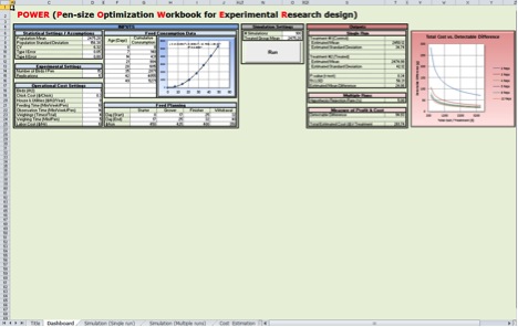 Figure 1. The “Dashboard” Worksheet: Tool Overview
How Are the Individual POWER for Poultry Worksheets Used?
The "Dashboard" worksheet contains input, run and output sections. All inputs should be entered on the "Dashboard" worksheet (Figure 2).
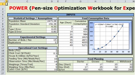 Figure 2. Set-up inputs - Part of the “Dashboard” Worksheet
- The population mean, standard deviation, Type I errors and Type II errors are input here. The example values of "Population Mean" and "Population Standard Deviation" are for a flock of female broilers when they were 48 days old (Shim et al., unpublished).
- The number of birds per pen and replications per treatment have to be entered. These two numbers will define the experiment you want to simulate.
- The current costs to conduct experiments have to be entered.
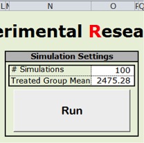 Figure 3. The “Run button” - Part of the “Dashboard” Worksheet
- Appropriate historical data should be entered under “Feed Consumption Data.” A graph is automatically adjusted and the coefficients are used to generate costs for different weights of birds.
- Lastly, there is a feed planning table to modify. This table is used to allocate feed charges for different times during the birds' life. Cost calculations will automatically be adjusted without any manual corrections to the other worksheets. For example, if you plan to use "Starter," "Grower," "Finisher" and "Withdrawal" feeds, just fill in the cells with the days that each feed will be fed and its cost. If you do not want to use grower feed, just empty the "Grower" column and only enter values into the "Starter," "Finisher" and "Withdrawal" feed columns.
- The number of simulations to be run and the mean for a treated group should be entered just above the "Run" button (Figure 3).
- Each time you want to simulate a new experiment, click the "Run” button.
- The results of one simulated experiment are displayed on the "Dashboard" under "Outputs" (Figure 4).
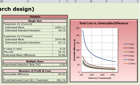 Figure 4. Reading Outputs - Part of the “Dashboard” Worksheet
The "Simulation (Single run)" worksheet shows a simulation to compare two treatments with each replication (Figure 5). In the example in Figure 5, each replicate contains 15 birds and each treatment contains five replicates. For example, cell B3 contains a randomly generated individual bird weight from a normal distribution with the mean and standard deviation input.
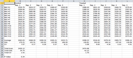 Figure 5. The “Simulation (Single run)” Worksheet showing the random bird values taken from the entered means and standard deviations
The "Simulation (Multiple runs)" worksheet shows multiple simulations (Figure 6). Each row shows one experiment. The cell B9 presents the average weight of one pen of randomly generated “birds.” The G9 and O9 cells present average weights of five pens each for the Control and Treated groups, respectively. The H9 and P9 cells present the corresponding standard deviations. These cells will change based on the number of replications. This worksheet also contains the average mean difference, t-statistic and P-values based on the number of replications. The last column is used to tabulate the number of individual simulations meeting the rejection rate probability. It is summed at the bottom of the page. It was an assumption for the simulation to see how accurate the result will be based on the input settings. If the mean values for the control and treated groups are identical, then the Hypothesis Rejection Rate (%) should be 5.0. In the example in Figure 4, it is 5.0. By clicking on the "Simulation" you can see how the P-values vary based on the assumption of a normal distribution for the population mean, like in a Monte-Carlo Simulation.
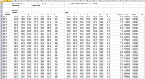 Figure 6. The “Simulation (Multiple runs)” Worksheet showing the random bird values taken from the entered means and standard deviations
The "Cost_Estimation" worksheet contains the calculation details for experimental costs (Figure 7). Every input value was from the "Dashboard." Values should not be overwritten on this sheet.
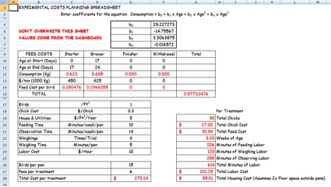 Figure 7. Cost_Estimation Worksheet
The "TC_vs_DD" worksheet displays total costs (from $366.40 to $3,505.33) and detectable differences against various numbers of birds per pen and replications, which make from 120 to 1,920 total birds (Figure 8). This worksheet contains the same graph as in the "Dashboard" and a graph of birds per pen (from five to 80) and detectable differences.
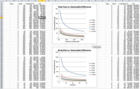 Figure 8. TC_vs_DD Worksheet
The "Chart 1" and "Chart 2" worksheets show the detectable difference versus total costs (Figure 9) and the detectable difference versus birds per pen (Figure 10) that are also displayed on the "TC_vs_DD" worksheet. These were included for printing.
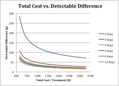 Figure 9. Chart 1 Worksheet
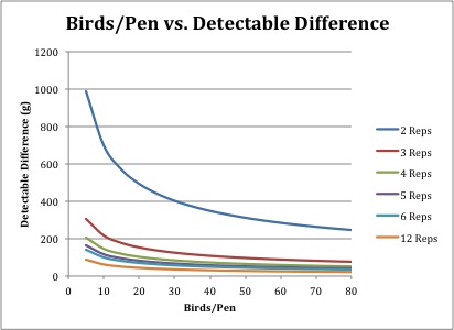 Figure 10. Chart 2 Worksheet
How Often Will Experimental Results Reflect Reality?
There is an easy test to demonstrate that the simulation model is working properly: When the Control and Treatments are input with identical means and standard errors, the null hypothesis that there were no differences in means should have a 5 percent rejection rate (P < 0.05) (Pesti and Shim, 2012). For example, the "Simulation (Multiple runs)" worksheet shows 5 percent rejection (Figure 6). Similar tests can be demonstrated for Type II error by running the problem with real differences between the control and treated groups and different levels of Type II error.
What Can Be Concluded from POWER for Poultry?
POWER analysis can be used to calculate the minimum sample size required so that one can be reasonably likely to detect an effect of a given size. In general, the larger the sample size, the smaller the sampling error tends to be. If the sample size is too small, there is not much point in gathering the data, because the results will tend to be too imprecise to be of much use. However, there is also a point of diminishing returns beyond which increasing sample size provides little benefit. Once the sample size is large enough to produce a reasonable level of accuracy, making it larger simply wastes time and money. Of course, each researcher has to decide what “reasonable” means and then accept that a certain percentage of the time their experiment will not yield the correct conclusions.
POWER calculations can be made whenever one performs a statistical test of a hypothesis and obtains a statistically non-significant result. Because of the very large amount of money at risk from declaring there were no significant differences in an experiment, there should be more information presented than the chance of declaring a significant difference when none exists. The detectable difference displayed on the ?Dashboard? sheet is from Zar (1981).
The number of replications required depends on the experimental design employed, the desired difference from the mean that one would like to be able to detect, and a specific probability level and type II error. The number of replications may be estimated using procedures described by Cochran and Cox (1957), Zar (1981) or Berndtson (1991).
When we assume that we use the same number of birds in an experiment (e.g., 600 total birds), the detectable differences decreases from 127.15 g to 27.78 g by going from two (300 birds per pen) to 12 (50 birds per pen) replications. This means that more replication numbers generally gives better results than more birds per pen. To estimate about 50 g detectable differences in 12 replications, 15 birds are needed. However, when replications were decreased from six to three, the number of birds per pen was increased from 40 to 185 to estimate about 50 g detectable difference.
With two replications per treatment, increasing the number of birds decreased the detectable differences very much. However, even with large numbers of birds per pen, the detectable differences were quite large (Figure 8). With 12 replications, the increase in the number of birds did not affect detectable differences nearly as much as with two replications, but did cause a steep increase in total costs.
In order to have a relatively small detectable difference with a reasonable cost, a proper trade-off study is necessary. POWER for poultry should be helpful for making the appropriate calculations and decisions.
Computational Requirement
This workbook runs on all modern versions of Microsoft Excel with the Visual Basic function. Macros need to be enabled. Download instructions for running the workbook here (PowerPoint).
References
Aaron, D.K. and V.W. Hays. 2004. How many pigs? Statistical power considerations in swine nutrition experiments. J. Anim. Sci. 82 (E. Suppl.): E245-E254.
Berndtson, W.E. 1991. A simple and reliable method for selecting or assessing the number of replicates for animal experiments. J. Anim. Sci. 69:67-76.
Cochran, W. G. and G. M. Cox. 1957. Experimental Designs, 2nd ed. John Wiley & Sons, New York. National Research Council, 1994. Nutrient Requirements of Poultry. 9th rev. ed. National Academy Press, Washington, DC.
Pesti, G. M. and M. Y. Shim. 2012. A spreadsheet to construct power curves and clarify the meaning of the word equivalent in evaluating experiments with poultry. Accepted to Poult. Sci.
SAS Institute, 2006. SAS User?s Guide: Statistics. Version 9.1.3 ed. SAS Inst. Inc., Cary, NC.
Shim, M. Y. and G. M. Pesti. 2012. Poultry Nutritionist Tool Kit. http://www.poultry.uga.edu/extension/Poultry-Nutrition.htm Accessed Aug. 2012.
Shim, M. Y., G. M. Pesti and M. Tahir. Unpublished. How many chickens? Statistical power considerations in experiments with poultry. The University of Georgia, Athens, GA 30602.
Zar, J. H. 1981. Power of statistical testing: Hypothesis about means. American Laboratory 13:102-107.
Status and Revision History
Published on Mar 31, 2013


